Popularly thought to be incomparable, apples and oranges have much more in common than you think. Beyond the fact that they’re both fruit, both can be easily compared in terms of price, taste, health benefits, etcetera, all of which indicators with which we use to compare the relative costs and benefits one fruit has over the other (depending on the person, of course. I personally prefer eating apples, but drinking orange juice.)
“different individuals have different preferences” – Charles Wheelan
Critics of Economics claim that the very basis of Economics, the assumption that individuals act to make themselves as well off as possible, is what makes the discipline pseudoscientific. Many economic models and theories presume that human preferences and economic conditions are universal and can be reduced to an equation or a mathematical model without subtlety, ambiguity or uncertainty, and thus, critics argue that such models lack the predictive power to correctly envision the economic future. However, experts in the discipline are not blind to this. Economics has continued to remain relevant as, to quote Robert Schiller, the discipline constantly evolves to “combine its mathematical insights with the kinds of adjustments that are needed to make its models fit the economy’s irreducibly human element.”
Before understanding how the discipline has evolved, we must first look at the very foundation of Economics that critics attack: rationality.
The discipline focuses on Instrumental Rationality, a specific form of rationality focusing on the most efficient or cost-effective means to achieve a specific end, but not in itself reflecting on the value of that end. In adopting the best actions to achieve one’s goal, an economic agent determines the options available, before choosing the most preferred one according to some consistent criterion that is typically based on self-interest.
To be able to compare the costs and benefits of options, we must adopt common accounting units, that allow us to linearly compare the characteristics of options (for instance, the prices, level of fibre or sweetness of apples and oranges). Much of Economics involves pegging a monetary value to all actions, be it the monetary value of time or of purchasing resources, allowing us to choose the most cost-effective option. This is the basis of Cost-Benefit Analysis (CBA), an appraisal method that provides analysis of social and economic gains and losses that could arise from a project. The aim of CBA is to put a monetary value on the benefits expected from the project and compare these to the costs which are expected to be incurred. If the benefit exceeds the cost, there is economic justification for the project to go ahead.
The following are three common forms of CBA that can be carried out during any economic endeavour (or decision-making):
- Ex Ante CBA refers to the more common use of the term CBA, to describe a project that is currently under consideration, but has not begun. Ex ante is used to assist the decision making and appraise the costs and benefits of a project.
- Ex Post CBA refers to a CBA carried out after a project has been completed. At this stage all of the costs are ‘sunk’, that is they have already been invested in the project. This type of project is therefore used primarily to assess the project contributing to ‘learning’, so that the information gathered can be used in assessing future projects.
- In Medias Res CBA term refers to CBAs that are carried out during a project, i.e after the project is already under way. This has the dual use of influencing the current project as with ex ante CBA, while also gathering information to inform future projects as with ex post CBA.
Understandably, it is difficult for everything to have a monetary value. We bring into question two scenarios:
Firstly, what about future monetary value? Many economic projects span a period of time to complete, thus an initial ex ante CBA might not hold true as the project progresses. With inflation and changes in cost due to market forces, the evaluation of a project’s costs will change over time.
This is where we introduce discounting: the process of determining the present value of a payment or a stream of payments that is to be received in the future. We discount future values in CBA to make costs & benefits when they occur across time algebraically comparable (i.e., so you can add them and subtract them). In order to discount, you need a discount rate, which is the interest rate you need to earn on a given amount of money today to end up with a given amount of money in the future. This accounts for the time value of money, which is the idea that a dollar today is worth more than a dollar tomorrow given that the dollar today has the capacity to earn interest.
For government CBA projects, we call the discount rate the Social Discount Rate (SDR). In general, a higher discount rate means that there is a greater the level of risk associated with an investment and its future cash flows, as it lowers the present value of the investment. Too high an SDR can mean under-investment in social programs due to an aversion to risk, and a smaller public sector. Too low an SDR can mean over-investment, and a larger public sector. Thus, discount rates can have ramifications that transcend the mathematics. By understanding the effects of inflation and changes in cost, discounting appropriately can allow economic agents to have greater certainty over the future, allowing them to continue making accurate CBAs now.

Secondly, what about non-market goods? These are goods and services that are not traditionally traded and do not have monetary value. What about the peanut-butter sandwich your mother made for you this morning? Or the impact of a sea-view versus a garden-view on the valuation of the price of a condominium?
This is where we introduce shadow pricing: the assignment of a dollar value to an abstract commodity that is not ordinarily quantifiable as having a market price, but needs to be assigned a valuation to conduct a cost-benefit analysis. A shadow price is assigned to goods that are not generally bought and sold as separate assets in a marketplace, such as production costs (the cost of your mother’s time, effort, etcetera in producing the sandwich) or intangible assets (the value of a view).
An example of shadow pricing as applied to a proposed plan to renovate a school’s facilities might be the assignment of a dollar value to the expected benefits of doing the renovation. While the cost of the renovation can be easily assigned a dollar value, there are elements of the project’s expected benefit that must be assigned a shadow price because they are difficult to quantify. The possible benefits of the project include improved student morale, a lower teacher turnover rate and increased productivity. Since it is impossible to assign a precise dollar value to such potential benefits, an estimated shadow price is assigned to set a dollar figure to compare to the cost figure.

Having understood the breadth of CBA, we see how various economic conditions can be brought together and compared linearly under a universal model. With the development of various common accounting units, discounting and shadow pricing, the comparing of various preferences has subtlety, and accounts for ambiguity and uncertainty. Thus, the rational economic agent becomes more believable – he has the tools to compare and weigh costs and benefits. However, the ability to compare is different from the ability to optimise – can the economic agent really maximise self-interest?
Let us assume a consumer has already weighed the marginal costs and benefits of consuming the next units of apples and oranges using CBA. The final step then, is to understand how much the consumer can afford (budget constraints), and what the consumer wants (preferences illustrated with indifference curves). This process of optimisation is known as Consumer Choice Theory (CCT).
CCT is the measure by which we derive an individual’s demand curve (aggregating the demand curves of all individuals gives you the market demand curve, which you can read up more on in H2: Inside-Out!). Assuming only two goods (apples and oranges), an individual will have multiple possible combinations of consumer expenditure. These choices, however, are limited by budget constraints.

The budget constraint curve is illustrated by the blue line in the above diagram. The slope of the budget constraint line equals the relative price of the two goods, that is, the price of one good compared to the price of the other. It measures the rate at which the consumer can trade one good for another, and is specific to the budget a consumer has. An increase in the consumer’s budget would result in a parallel outward shift of the blue line.
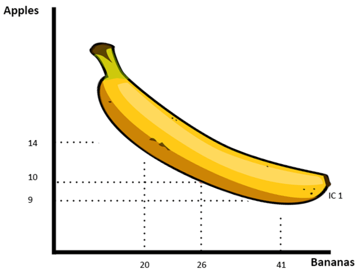
The indifference curve represents combinations of goods which the consumer has equal preference for, as each combination gives the same level of satisfaction (thus the consumer is indifferent or happy with all of the points on the same curve). These are represented by IC1, IC2 and IC3 in the above diagram. The slope at any point on an indifference curve is known as the marginal rate of substitution – the rate at which a consumer is willing to trade one good for another (similar to the budget constraint curve)
The properties and assumptions of indifference curves are as follows:
- Higher indifference curves are preferred to lower ones (IC2 is preferred to IC1 is preferred to IC3). This is because consumers would usually prefer more of something to less of it, and higher indifference curves represent larger quantities of goods than lower indifference curves.
- Indifference curves are downward sloping. A consumer is willing to give up one good only if he gets more of the other good to remain equally happy.
- Indifference curves are convex to the axis. This is due to the law of diminishing marginal utility and increasing opportunity cost (see H2: Inside-Out!). Or, it can be seen as people are more willing to trade away goods that they have an abundance in and less willing to trade away goods of which they have little. These are caused by differences in marginal substitution rates at each point.
- Indifference curves do not cross. Looking at the diagram below, the blue curve tells us that consuming 2 oranges and 3 apples (A) gives the consumer the same utility as consuming 4 oranges and 2 apples (B). However, the red curve tells us that consuming 4 oranges and 2 apples (B) would give the consumer the same utility as consuming 3 oranges and 3 apples (C). This implies that consuming 2 oranges and 3 apples would give the same utility as consuming 3 oranges and 3 apples (A = C, since A = B and B = C). However, C > A, given the assumption that consumers would usually prefer more of something to less of it. Thus, indifference curves cannot share points, and thus cannot cross.

Optimisation would be to get the combination of goods on the highest possible indifference curve, but at the same time, the consumer must also end up on or below his budget constraint. The optimal point would be where the consumer’s marginal rate of substitution equals the relative price (or where the highest indifference curve and budget constraint are tangent). Thus, any point on IC2 would be desirable, but unattainable, as it is above his budget constraint. Any point on IC3 would be desirable and attainable, but sub-optimal. The optimal point would be the red point on IC1.
Should there be a change in the price of one good relative to another, the slope of the budget constraint changes, shifting to reflect the new relative prices. However, the process of determining the optimal point of consumption remains the same, just that a new optimal point will be chosen in which one good is consumed more than before (the one whose price fell relative to the other), and the other good is consumed less than before (the one whose price rose relative to the other). This is due to the income effect (when a good takes up a higher proportion of income and less of it is consumed) and the substitution effect (when close and available substitutes become relatively more affordable, and consumers switch to them).
Understanding CBA and CCT allows us to understand how economic agents weigh their costs and benefits, and how they optimise to maximise self-interest. These form the tenets of Rational Choice Theory. From our analysis, we see that Rational Choice Theory paints an image of a rational consumer that has the following:
- Complete Preferences (perfect knowledge of one’s own tastes and preferences)
- Transistive Preferences (If A > B, and B > C, then A > C)
- Context-Independent Preferences (different circumstances and situations do not change one’s preferences)
- Stable Preferences (preferences do not change over time)
So admittedly, Rational Choice Theory has its flaws. Decision-making models fail because preferences are never always complete, transistive, context-independent or stable, which leads to bounded rationality, or rationality that is limited by a lack of information, cognitive ability or time. However, the discipline has evolved to account for a world which isn’t perfect, such that within the limitations of human time, intelligence and resources, we can use these tools to weigh our costs and benefits, and maximise self-interest.
So the next time someone advises you against comparing apples and oranges, approach the situation rationally. Or get a banana instead – I heard they’re a great source of potassium.

You must be logged in to post a comment.